
Game of Thrones certainly does not need any introduction. It is one of the highly popular shows with record breaking viewership of 17.4 million people who tuned in last sunday for the final season premiere as reported by Fortune yesterday. However the trend of growing viewership has been consistently observed in every season.
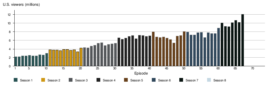
From the above image (taken from Wikipedia) you can clearly see that Season-1 had around 2 million consistent viewership where as Season-7 has over 12 million in viewership. As the show has grown, so has the production budget per episode. During Season-2, each episode cost an average of 6 million USD to produce, but this figure jumped to 10 million USD by Season-6. Based on a report from Vanity Fair it seems each episode in Season-8 (last season) costs around 15 million USD for production. The show is also one of the highly acclaimed one during awards season and it has been nominated for two Golden Globes in 2017. In 2016 alone, the show won 12 Primetime Emmy Awards, making it the Emmy’s second most successful TV series of all time.
In this blog article, we will run through some data visualizations about how importance of certain characters changed during the course of seasons, how the death trends changed over all seasons and finally we do survival analysis on alive characters, build a model to predict their survival chances in Season-8. The model just provides an estimate based on previous trends observed, but does not guarantee if its to happen for sure. You know how the GoT took every one by its twists and surprises, who would have guessed Eddard Stark would die so soon, right?
Data
The original data comes from this github user @jeffreylancaster who has done an amazing job of compiling all the data scene by scene and for all seasons.
But this data is in json format, so we transform it to csv which is more usable for our analysis, and also in the process, we create some additional information for every character such as their screen times in every season, number of people they killed per season, eigenvector centrality based on screen time in every season etc.
The final transformed data (csv) is published in this github repository
Important Characters
In this section, we run through a series of data visualizations about how certain character’s importance changed through the course of seasons.
First we analyze each character’s importance primarily by two factors - total screen time in the season and
eigenvector centrality (ec) which is directly the measure of influence of the character in the whole network of interactions.
We build the network of interactions combining all scenes in a given season using networkx
and then derive ec scores at every character (node) in the network using edge screen time as weight. The edge screen time is the total
season’s screen time shared with a particular character. In Chart-1 below, x-axis represents the total screen time
in the given season where as y-axis represents the ec score in the season. In other words, bubbles (characters) tend to be right-side when they have
more screen time and towards left-side when they don’t have much screen time. Similarly, the bubbles (characters) tend to move upwards
when they have relatively more influence on the network and if they tend to bee downwards, that’s when they do not have much influence.
You may use the control buttons/slider at the bottom of this chart to navigate through the seasons.
Few observations from the above chart:
- In Season-1, Stark’s pretty much dominated the scene with Eddard Stark having season’s maximum around 142 mins (2.3 hrs) of screen time. Eddard in season-1 also has more influence. The other members of Stark family such as Catelyn, Arya, Rob, Bran, Sansa, Jon Snow also dominated the season’s landscape with considerable influence as well. Of all the Lannisters, Tyrion has more screen time but not much influence. Cersei Lannister, Robert Baratheon and Joffrey Baratheon also have considerable screen times and influence.
- In Season-2, most of the Stark members dropped both in terms of screen time as well as influence, how ever Sansa still has a considerable influence. Tyrion Lannister has more screen time and more influence in this season. Joffrey and Cersei also have better influence.
- In Season-3, most of the character’s have dropped their influence. Catelyn and Robb have highest influence. Also, we see few Tully’s and Frey’s started to gain more influence.
- In Season-4, its all about Lannisters show. Tyrion, Tywin, Cersei and Jaime all have greater influence and more screen times as well. Sansa still has some influence probably she is married into Lannisters while other Starks dropped. We see Tyrell group rising to some influence a little bit.
- In Season-5, Jon Snow dominated in screen time but not on the influence though. Cersei also has considerable screen time but not much influence. Tyrion Lannister, Daenerys Targaryen and Jorah Mormont have the highest influence in this season.
- In Season-6, Starks (Jon Snow and Sansa) took some charge again both in terms of screen time and influence. Tyrion Lannister’s and Daenerys Targaryen’s influence dropped in this season.
- In Season-7, Jon Snow is still in the lead in terms of screen time and influence. Tyrion and Daenerys gained both influence and screen time. Jaime and Cersei also gained some influence.
In Chart-2 below, we see the overall screen time with all season’s combined. Hover over individual bars to reveal detailed information.
Few observations from the above chart:
- Tyrion Lannister shares the maximum screen time overall with 549 mins (9.15 hrs) and second to him is Jon Snow who has 547 mins (9.11 hrs).
- Daenerys Targaryen, Cersei Lannister and Sansa Stark are next in the line with 420 mins (7 hrs), 399 mins (6.65 hrs) and 362 mins (6.05 hrs) respectively.
- Arya Stark has 332 mins (5.54 hrs) and Jaime Lannister has 329 mins (5.48 hrs).
Death Toll Trends
In this section, we run through some more visualizations but this time on the character death trends.
In Chart-3 below, we see the death count (y-axis) by season (x-axis). Please hover over bars for more information. We see the death took its toll by Season-6 with death count of 50 characters. Please note that only prominent characters with considerable screen time have been included in this count.
Below is the list of important characters (not the exhaustive list) who were dead in every season:
- Season-1: Viserys Targaryen, Robert Baratheon, Eddard Stark, Khal Drogo
- Season-2: Renly Baratheon, Alton Lannister.
- Season-3: Richard Karstark, Robb Stark, Catelyn Stark
- Season-4: Joffrey Baratheon, Lysa Arryn, Oberyn Martell, Shae, Tywin Lannister
- Season-5: Master Aemon, Shrine Baratheon, Selyse Baratheon, Stannis Baratheon, Myrcella Baratheon
- Season-6: Doran Martell, Trystane Martell, Roose Bolton, Walda Bolton, Balon Greyjoy, Aerys Targaryen, Brynden Tully, Rickon Stark, Ramsay Bolton, Lancel Lannister, Margaery Tyrell, Loras Tyrell, Mace Tyrell, Kevan Lannister, Tommen Baratheon.
- Season-7: Ellaria Sand, Several members of House Frey, Lady Olenna, Randyll and Dickon Tarly, Thoros of Myr, Benjen Stark.
Who killed the most?
In Chart-4 below, we see the number of people killed (y-axis) by each character (x-axis). Please hover over bars for more information. Clearly, we can see that Daenerys Targaryen and Jon Snow killed the maximum people. Arya Stark killed 9 people and Cersei Lannister killed 7 people.
How are they killed?
So how are these people killed? In Chart-5 below, we see the number of people killed (y-axis) by manner of death (x-axis). We see most common ways people are being killed are Multiple stabs (14), Chest stabs (12), Throat slash (11) and Decapitation (10)
Here are the most common ways used by Daenerys Targaryen, Jon Snow, Arya Stark, Cersei Lannister to kill people,
df2 = character_df[(character_df.killed_by.notnull()) & (character_df.killed_by.str.contains('Daenerys Targaryen')) ]
df2 = DplyFrame(df2) >> sift(X.manner_of_death.notnull()) >> group_by(X.manner_of_death) >> summarize(total=X.character_name.count())
print('Daenerys Targaryen: ', list(df2['manner_of_death'].unique()))

df2 = character_df[(character_df.killed_by.notnull()) & (character_df.killed_by.str.contains('Jon Snow')) ]
df2 = DplyFrame(df2) >> sift(X.manner_of_death.notnull()) >> group_by(X.manner_of_death) >> summarize(total=X.character_name.count())
print('Jon Snow: ' , list(df2['manner_of_death'].unique()))

df2 = character_df[(character_df.killed_by.notnull()) & (character_df.killed_by.str.contains('Arya Stark')) ]
df2 = DplyFrame(df2) >> sift(X.manner_of_death.notnull()) >> group_by(X.manner_of_death) >> summarize(total=X.character_name.count())
print('Arya Stark: ' , list(df2['manner_of_death'].unique()))

df2 = character_df[(character_df.killed_by.notnull()) & (character_df.killed_by.str.contains('Cersei Lannister')) ]
df2 = DplyFrame(df2) >> sift(X.manner_of_death.notnull()) >> group_by(X.manner_of_death) >> summarize(total=X.character_name.count())
print('Cersei Lannister: ' , list(df2['manner_of_death'].unique()))
Daenerys Targaryen:  ['Burning', 'Dragon', 'Safe']
Jon Snow:  ['Arrow', 'Burning', 'Chest stab', 'Decapitation', 'Face stab', 'Head crush']
Arya Stark:  ['Chest stab', 'Multiple stabs', 'Neck stab', 'Throat slash']
Cersei Lannister:  ['Poison', 'Wildfire']
Death Trends in various groups
Chart-6 below is a series of sub plots each one specifying death percentage by group under consideration.
Few observations from the above chart:
- About 52% of all male characters are dead while only 33% of female are dead.
- The houses of Arryn, Bolton and Tyrell are completely gone. Lannisters suffer from 60% death rate, while Starks have 45%. Targaryens have a low death rate of 27%.
- About 38% of royals are dead and about 45% of those who are not royals are dead.
- About 50% of kingsguard’s are dead while 44% of those who are not kingsguard are dead.
Survival Analysis
I know you are bored to death with visualizations by now, so lets go straight to the purpose of this post here.
Background
From Wikipedia defines survival analysis as below,
a branch of statistics that deals with analysis of time duration until one or more events happen, such as death in biological organisms and failure in mechanical systems.
Survival Analysis is also called as Time-to-Event Analysis. It was primarily designed for healthcare domain where it was used to predict the survival rate of patients when they are given some medical treatment. But this can be applied to a wide variety of business use cases some of them are listed below:
- Customer Retention: Here we predict if a particular customer unsubscribe from our service or cancels their account with our business. By making these predictions, it would help the business to tailor some marketing offer exclusively to these folks and make some efforts to keep them in business.
- Predictive Maintenance: Here we predict how long certain machines run without problems, for e.g, aircraft engines etc. Thus, we can plan service events accordingly so as to bring the machine back to normal.
Below image illustrates the idea of survival analysis,
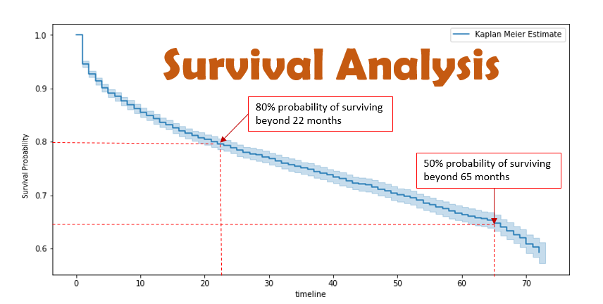
Sometimes for certain data points in the study we may not see their time-to-event as they might actually occur outside the study period. Such data points are called censored. It can be right-censored or left-censored depending on whether the event occurs after our study period or before our study period. If we choose not to include the censored data, then it is highly likely that our estimates would be highly biased and under-estimated. The inclusion of censored data to calculate the estimates, makes the Survival Analysis very powerful, and it stands out as compared to many other statistical techniques.
Theory
If you cannot spare the math here, you may jump directly to the section, Kaplan-Meier Model Estimate for GoT characters
The survival function, \(S(t)\), of an individual is the probability that they survive until at least time \(t\).
\[S(t) = \Pr(T > t)\]where \(t\) is a time of interest and \(T\) is the time of event.
The survival curve is non-increasing function as the the event of interest will not reoccur for an individual and is limited within the range \([0,1]\). Note that the event might not happen within our period of study and we call this right-censoring.
The hazard function \(\lambda(t)\) is a related measure, telling us the probability that the event \(T\) occurs in the next instant \(t + \delta t\), given that the individual has reached time \(t\):
\[\lambda(t) = \lim_{\delta t \rightarrow 0} \frac{\Pr(t \leq T < t + \delta t \ | \ T > t)}{\delta t}\]The above equation can be worked back to the Survival function:
\[S(t) = exp(- \int\limits_{0}^{t} \lambda(u)du)\]The hazard function is non-parametric, so we can fit a pattern of events that is not necessarily monotonic.
The cumulative hazard function is an alternative representation of the time-to-event behaviour , which is essentially the summing of the hazard function over time, and is used by some models for its greater stability.
Further we can show the relation between hazard function and survival function as below,
\[\Lambda(t) = \int\limits_{0}^{t} \lambda(u)du = -\log S(t)\]which can be rewritten as below,
\[S(t) = -e^{\sum \Lambda_i(t)}\]The survival analysis methods can be broadly classified into two groups: non-parametric and parametric.
Kaplan-Meier Model is the most simplest model which keeps track of event tables. This model gives us a maximum-likelihood estimate of the survival function,
\[\hat S(t) = \prod\limits_{t_i \\< t} \frac{n_i - d_i}{n_i}\]where \(d\) and \(n\) are respectively the count of ‘death’ events and individuals at risk at time \(i\).
The cumulative product gives us a non-increasing curve where we can read off, at any time step during the study, the estimated probability of survival from the start to that time step. While this approach is interesting, it has its own limitations that the other characteristics of data points are not taken into consideration.
Cox Proportional Hazards Model or simply called as Cox PH model gives a semi-parametric method of estimating the hazard function at time \(t\) given a baseline hazard that’s modified by a set of covariates:
\[\lambda(t|X) = \lambda_0(t)\exp(\beta_1X_1 + \cdots + \beta_pX_p) = \lambda_0(t)\exp(\bf{\beta}\bf{X})\]where \(\lambda_0(t)\) is the non-parametric baseline hazard function and \(\bf{\beta}\bf{X}\) is a linear parametric model using features of the individuals, transformed by an exponential function.
For our analysis further, we would utilize both KM and Cox PH approaches.
Kaplan-Meier Model Estimate for GoT characters
Data Preparation
Since KM model is non-parametric we load the data as is, no additional information is derived.
data_path = '/Users/genie/dev/projects/github/got_survival_analysis/data/got_characters_s1_to_s7.csv'
character_df = pd.read_csv(data_path,quotechar='"',na_values='',encoding = "ISO-8859-1")
As mentioned above in the theory, KM model cares about only two features - durations and event observed which in our case are mentioned below:
- duration_in_episodes value for every character is defined as the total number of episodes elapsed until the character actually dies. Every character’s duration counter gets incremented after every passing episode if they are not dead in the episode irrespective of whether the character shares any screen time or not in the episode. For those are dead in the episode, the counter concludes. For example if someone dies in episode 54, their duration_in_episodes=54 while for others who are alive, it continues to increment. By default, every alive character at the end of Season-7 have duration_in_episodes=67 because there are a total of 67 episodes all seasons combined so far.
- is_dead value is an indicator whether the character is dead or alive.
Build KM Model
We utilize a python package called lifelines which provides implementations for several survival analysis.
We create a KaplanMeierFitter object and fit the model to our data as shown below,
from lifelines import KaplanMeierFitter
kmf = KaplanMeierFitter()
kmf.fit(durations = character_df.duration_in_episodes, event_observed = character_df.is_dead)
<lifelines.KaplanMeierFitter: fitted with 368 observations, 203 censored>
Then using the code below we can look into the event table that KM model keeps track of,
kmf.event_table
          removed  observed  censored  entrance  at_risk
event_at
0.0             0         0         0       368      368
1.0             5         5         0         0      368
2.0             3         3         0         0      363
5.0             2         2         0         0      360
6.0             4         4         0         0      358
7.0             1         1         0         0      354
8.0             5         5         0         0      353
9.0             1         1         0         0      348
10.0            4         4         0         0      347
11.0            1         1         0         0      343
12.0            1         1         0         0      342
13.0            2         2         0         0      341
15.0            2         2         0         0      339
16.0            4         4         0         0      337
17.0            7         7         0         0      333
19.0            2         2         0         0      326
20.0            6         6         0         0      324
23.0            1         1         0         0      318
24.0            3         3         0         0      317
25.0            4         4         0         0      314
26.0            1         1         0         0      310
28.0            2         2         0         0      309
29.0            4         4         0         0      307
30.0            2         2         0         0      303
31.0            1         1         0         0      301
33.0            2         2         0         0      300
35.0            3         3         0         0      298
37.0            3         3         0         0      295
38.0            2         2         0         0      292
39.0            3         3         0         0      290
40.0            6         6         0         0      287
41.0            2         2         0         0      281
42.0            1         1         0         0      279
43.0            1         1         0         0      278
44.0            2         2         0         0      277
45.0            2         2         0         0      275
47.0            1         1         0         0      273
48.0            3         3         0         0      272
49.0            2         2         0         0      269
50.0            4         4         0         0      267
51.0            4         4         0         0      263
52.0            5         5         0         0      259
53.0            6         6         0         0      254
54.0            6         6         0         0      248
55.0            6         6         0         0      242
57.0            1         1         0         0      236
58.0            5         5         0         0      235
59.0            6         6         0         0      230
60.0           11        11         0         0      224
62.0            2         2         0         0      213
63.0            2         2         0         0      211
65.0            2         2         0         0      209
66.0            2         2         0         0      207
67.0          205         2       203         0      205
Some notes on the event table are as below:
- The removed column contains the number of observations removed during that time period, whether due to death (the value in the observed column) or censorship. So the removed column is just the sum of the observed and censorship columns. The entrance column tells us whether any new subjects entered the population at that time period. Since all the characters we are studying start at time=0, the entrance value is 368 at that time and 0 for all other times.
- The at_risk column contains the number of subjects that are still alive during a given time. The value for at_risk at time=0, is just equal to the entrance value. For the remaining time periods, the at_risk value is equal to the difference between the time previous period’s at_risk value and removed value, plus the current period’s entrance value. For example for time=1, the number of subject’s at risk is 363 which is equal to 368 (the previous at_risk value) - 5 (the previous removed value) + 0 (the current period’s entrance value).
By recalling the KM model equation mentioned in the previous section, We can define the survival probability for an individual time period as follows:
\[\hat S(t) = \frac{atrisk_t - died_t}{atrisk_t}\]For example at time=1, we calculate as below: \(\hat S_1 = \frac{368 - 5}{368} = 0.98\)
So, at the end of first episode (t=1), survival probability of a character is 98%. Similarly at the end of tenth episode (t=10), survival probability is simply the product of all individual survival probabilities at all prior time events, which can be simply calculated from the model as shown below:
km.predict(10)
0.9320652173913037
which means that there is a 93% chance that a character survives after the tenth episode.
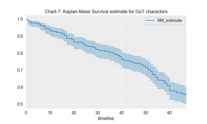
Since there are a total of 67 episodes all seasons combines, we calculate the survival probability at the end of 67th episode as below,
km.predict(67)
0.5516304347826084
We see that there is a 55% chance of survival for a character after 67th episode.
Survival Estimate ~ Overall
The overall survival probability estimate from KM model is as plotted below,
kmf.plot_survival_function()
Survival Estimate for selected groups
The next series of charts (from Chart-8 to Chart-11) represent the survival probabilities for the desired groups under study such as males vs females, royals vs non-royals, kingsguard vs non-kingsguard, houses of allegiance
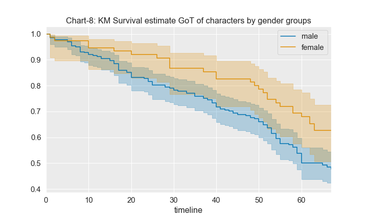
From the chart above, we understand that the survival chances for females is better than that of males at any given point in time.
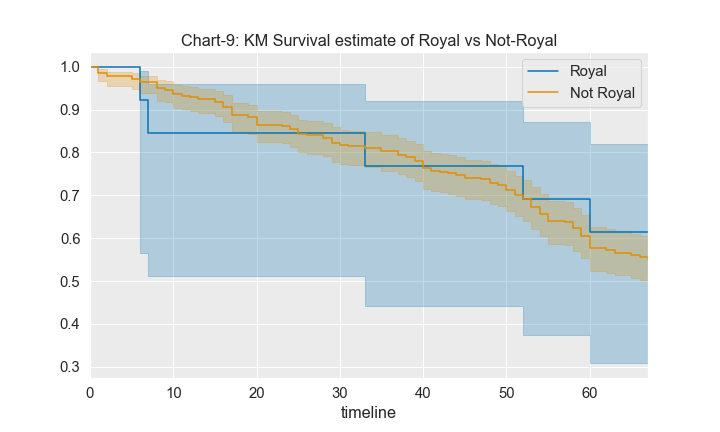
From the chart above, we understand that the survival chances for royals dropped over time though it was good for certain periods of time, where as for not-royals, it dropped consistently.
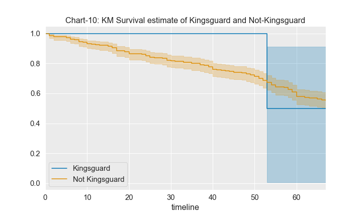
From the chart above, we understand that the survival chances for kingsguard is pretty much high until around 50-53 episode but after that it dropped drastically. However for non-kingsguard, it consistenly dropped over time.
Similarly, we plot for various houses,
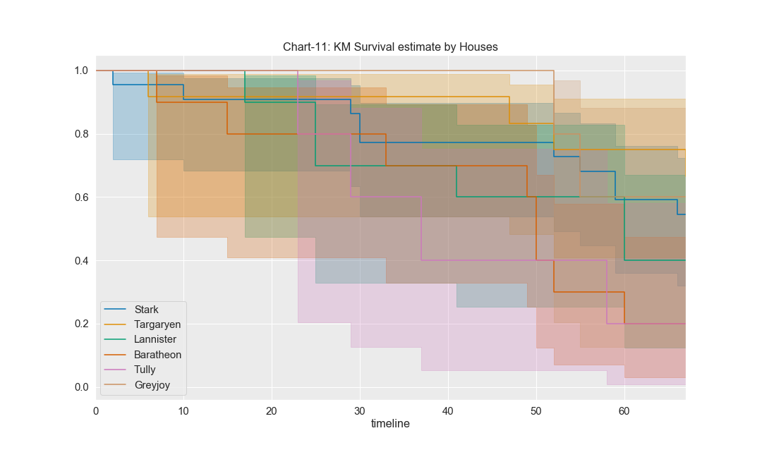
Few observations from above chart:
- Greyjoys have the highest chances of survival, nearly 80%
- Targaryens and Starks have about 60% chances of survival.
- Lannisters have around 40% chances of survival.
- Tullys and Baratheons have the lowest chances of survival of about 20%
Cox Proportional Hazard (PH) Model Estimate for GoT characters
Data Preparation
As mentioned in theory earlier that unlike Kaplan-Meier estimate, Cox PH considers wide range of features from the data points for making predictions, essentially its a regression. Hence we also derive some additional features for the data points, for example for a given character we derive additional information such as total screen time, number of people killed, is married or not, have guardian or not, have dead relatives?, have dead allies? etc.
Also Cox PH model needs all categorical variables to be converted to a dummy/indicator form.
Below is some code excerpt used for transforming and preparing the dataset for Cox PH model,
data_path = '/Users/genie/dev/projects/github/got_survival_analysis/data/got_characters_s1_to_s7.csv'
character_df = pd.read_csv(data_path,quotechar='"',na_values='',encoding = "ISO-8859-1")

character_df['total_screen_time'] = character_df.apply(lambda x: sum([x['s'+str(i)+'_screenTime'] for i in range(1,8)]), axis=1)
character_df['num_of_episodes_appeared'] = character_df.apply(lambda x: sum([x['s'+str(i)+'_episodes'] for i in range(1,8)]), axis=1)
character_df['num_of_people_killed'] = character_df.apply(lambda x: sum([x['s'+str(i)+'_numKilled'] for i in range(1,8)]), axis=1)
character_df['is_married'] = character_df.apply(lambda x: (0 if x['spouse']=='' else 1), axis=1)
character_df['have_siblings'] = character_df.apply(lambda x: (0 if x['siblings']=='' else 1), axis=1)
character_df['have_children'] = character_df.apply(lambda x: (0 if x['parent_of']=='' else 1), axis=1)
character_df['is_guardian_for_any'] = character_df.apply(lambda x: (0 if x['guardian_of']=='' else 1), axis=1)
character_df['is_guarded_by_any'] = character_df.apply(lambda x: (0 if x['guarded_by']=='' else 1), axis=1)
character_df['is_served_by_any'] = character_df.apply(lambda x: (0 if x['served_by']=='' else 1), axis=1)
character_df['serves_any'] = character_df.apply(lambda x: (0 if x['serves']=='' else 1), axis=1)
character_df['have_allies'] = character_df.apply(lambda x: (0 if x['allies']=='' else 1), axis=1)

dead_characters = list(character_df[character_df.is_dead==1]['character_name'].values)

def derive_if_have_any_dead_relatives(x):
    for p in x['spouse'].split(';'):
        if p in dead_characters:
            return(1)
    for p in x['parents'].split(';'):
        if p in dead_characters:
            return(1)
    for p in x['siblings'].split(';'):
        if p in dead_characters:
            return(1)
    for p in x['parent_of'].split(';'):
        if p in dead_characters:
            return(1)
    return(0)

def derive_if_have_any_allies_dead(x):
    for p in x['allies'].split(';'):
        if p in dead_characters:
            return(1)
    return(0)

character_df['have_dead_relatives'] = character_df.apply(derive_if_have_any_dead_relatives, axis=1)
character_df['have_dead_allies'] = character_df.apply(derive_if_have_any_allies_dead, axis=1)

# remove unwanted variables
character_df = character_df.drop(['s'+str(i)+'_screenTime' for i in range(1,8)], axis=1)
character_df = character_df.drop(['s'+str(i)+'_shareOfScreenTime' for i in range(1,8)], axis=1)
character_df = character_df.drop(['s'+str(i)+'_episodes' for i in range(1,8)], axis=1)
character_df = character_df.drop(['s'+str(i)+'_numKilled' for i in range(1,8)], axis=1)
character_df = character_df.drop(['spouse','parents','siblings','parent_of','manner_of_death',
                                  'killed_by','dead_in_season','guardian_of','guarded_by',
                                  'served_by','serves','allies'], axis=1)

df_r = character_df.drop(['character_name'], axis=1)
df_r.house = df_r.house.fillna('')
df_r['house_Stark'] = [(1 if 'Stark' in item else 0) for item in df_r['house']]
df_r['house_Lannister'] = [(1 if 'Lannister' in item else 0) for item in df_r['house']]
df_r['house_Targaryen'] = [(1 if 'Targaryen' in item else 0) for item in df_r['house']]
df_r['house_Bolton'] = [(1 if 'Bolton' in item else 0) for item in df_r['house']]
df_r['house_Greyjoy'] = [(1 if 'Greyjoy' in item else 0) for item in df_r['house']]
df_r['house_Martell'] = [(1 if 'Martell' in item else 0) for item in df_r['house']]
df_r['house_Mormont'] = [(1 if 'Mormont' in item else 0) for item in df_r['house']]
df_r['house_Tarly'] = [(1 if 'Tarly' in item else 0) for item in df_r['house']]
df_r['house_Tully'] = [(1 if 'Tully' in item else 0) for item in df_r['house']]
# df_r['house_Tyrell'] = [(1 if 'Tyrell' in item else 0) for item in df_r['house']]
df_r = df_r.drop(['house'], axis=1)

# removing unwanted variables
df_r = df_r.drop(['s'+str(i)+'_ec' for i in range(1,8)], axis=1)
df_r = df_r.drop(['s'+str(i)+'_bc' for i in range(1,8)], axis=1)

df_dummy = pd.get_dummies(df_r, drop_first=True)
Here is the final list of variables for the dataset,
df_dummy.info()
<class 'pandas.core.frame.DataFrame'>
RangeIndex: 368 entries, 0 to 367
Data columns (total 35 columns):
royal                               368 non-null int64
kingsguard                          368 non-null int64
s1_numOfCharactersInteractedWith    368 non-null int64
s2_numOfCharactersInteractedWith    368 non-null int64
s3_numOfCharactersInteractedWith    368 non-null int64
s4_numOfCharactersInteractedWith    368 non-null int64
s5_numOfCharactersInteractedWith    368 non-null int64
s6_numOfCharactersInteractedWith    368 non-null int64
s7_numOfCharactersInteractedWith    368 non-null int64
is_dead                             368 non-null int64
duration_in_episodes                368 non-null int64
total_screen_time                   368 non-null float64
num_of_episodes_appeared            368 non-null int64
num_of_people_killed                368 non-null int64
is_married                          368 non-null int64
have_siblings                       368 non-null int64
have_children                       368 non-null int64
is_guardian_for_any                 368 non-null int64
is_guarded_by_any                   368 non-null int64
is_served_by_any                    368 non-null int64
serves_any                          368 non-null int64
have_allies                         368 non-null int64
have_dead_relatives                 368 non-null int64
have_dead_allies                    368 non-null int64
house_Stark                         368 non-null int64
house_Lannister                     368 non-null int64
house_Targaryen                     368 non-null int64
house_Bolton                        368 non-null int64
house_Greyjoy                       368 non-null int64
house_Martell                       368 non-null int64
house_Mormont                       368 non-null int64
house_Tarly                         368 non-null int64
house_Tully                         368 non-null int64
house_Tyrell                        368 non-null int64
gender_male                         368 non-null uint8
dtypes: float64(1), int64(33), uint8(1)
memory usage: 98.2 KB
Build Cox PH Model
Before we proceed to build the model, let us observe if there is any correlation between variables. This can be done using a simple correlation matrix.
corr = df_dummy.corr()
ax = plt.axes()
sns.heatmap(corr,ax = ax,xticklabels=corr.columns,yticklabels=corr.columns,cmap='Blues')
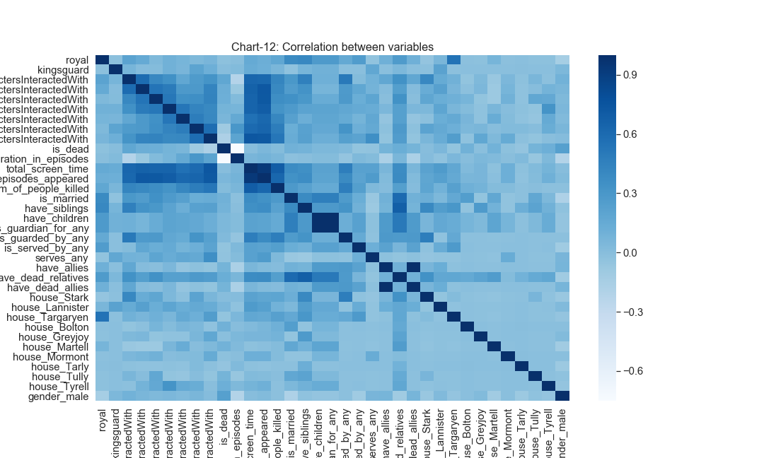
From the chart above, we observe that there is high correlation between the following variable pairs, (have_allies, have_dead_allies), (have_children, is_guardian_for_any), (total_screen_time, number_of_episodes_appeared)
So we will have to get rid of atleast one in evary variable pair. Thus we drop the following variables have_allies, have_chidren, number_of_episodes_appeared.
Additionally we also drop following variables house_Bolton, house_Tyrell, house_Tarly were dropped because of their low variance which are causing convergence problems for the model.
df_dummy = df_dummy.drop(['num_of_episodes_appeared','have_allies','have_children','have_siblings','house_Bolton','house_Tyrell','house_Tarly'], axis=1)
Then, we build the model using lifelines package in python.
from lifelines import CoxPHFitter
cph = CoxPHFitter()
cph.fit(df_dummy, 'duration_in_episodes', event_col='is_dead')
cph.print_summary()
<lifelines.CoxPHFitter: fitted with 368 observations, 203 censored>
      duration col = 'duration_in_episodes'
         event col = 'is_dead'
number of subjects = 368
  number of events = 165
    log-likelihood = -877.34
  time fit was run = 2019-04-17 05:03:21 UTC

---
                                  coef exp(coef)  se(coef)     z      p  -log2(p)  lower 0.95  upper 0.95
royal                            -1.31      0.27      0.64 -2.06   0.04      4.66       -2.56       -0.06
kingsguard                        1.00      2.73      1.12  0.90   0.37      1.44       -1.19        3.19
s1_numOfCharactersInteractedWith  0.06      1.06      0.01  4.12 <0.005     14.70        0.03        0.09
s2_numOfCharactersInteractedWith  0.03      1.03      0.02  1.09   0.28      1.86       -0.02        0.07
s3_numOfCharactersInteractedWith  0.02      1.02      0.02  0.70   0.48      1.06       -0.03        0.07
s4_numOfCharactersInteractedWith  0.01      1.01      0.02  0.54   0.59      0.77       -0.02        0.04
s5_numOfCharactersInteractedWith  0.01      1.01      0.02  0.69   0.49      1.03       -0.03        0.06
s6_numOfCharactersInteractedWith -0.07      0.94      0.02 -2.92 <0.005      8.15       -0.11       -0.02
s7_numOfCharactersInteractedWith -0.11      0.90      0.03 -3.51 <0.005     11.10       -0.17       -0.05
total_screen_time                -0.00      1.00      0.00 -1.04   0.30      1.75       -0.01        0.00
num_of_people_killed              0.19      1.21      0.10  1.87   0.06      4.01       -0.01        0.38
is_married                        0.35      1.43      0.35  1.02   0.31      1.71       -0.32        1.03
have_siblings                    -0.23      0.80      0.39 -0.58   0.56      0.84       -0.99        0.54
is_guardian_for_any              -0.14      0.87      0.33 -0.42   0.67      0.57       -0.79        0.51
is_guarded_by_any                 0.29      1.33      0.72  0.40   0.69      0.53       -1.12        1.69
is_served_by_any                 -1.34      0.26      1.37 -0.98   0.33      1.61       -4.02        1.34
serves_any                        0.09      1.09      0.55  0.16   0.87      0.20       -0.99        1.16
have_dead_relatives               0.32      1.38      0.31  1.04   0.30      1.74       -0.29        0.94
have_dead_allies                  0.94      2.56      0.70  1.34   0.18      2.48       -0.43        2.31
house_Stark                      -0.84      0.43      0.56 -1.51   0.13      2.93       -1.94        0.25
house_Lannister                   0.96      2.61      0.55  1.75   0.08      3.65       -0.11        2.03
house_Targaryen                   0.99      2.70      0.59  1.69   0.09      3.44       -0.16        2.15
house_Greyjoy                     0.44      1.56      0.82  0.54   0.59      0.77       -1.16        2.04
house_Martell                     1.08      2.94      0.50  2.18   0.03      5.08        0.11        2.05
house_Mormont                     0.76      2.14      1.06  0.72   0.47      1.08       -1.31        2.83
house_Tully                       0.75      2.12      0.63  1.19   0.23      2.09       -0.49        1.99
gender_male                       0.83      2.30      0.22  3.75 <0.005     12.45        0.40        1.27
---
Concordance = 0.73
Log-likelihood ratio test = 107.11 on 27 df, -log2(p)=35.78
We can see each variable’s contribution in a plot below,
cph.plot()
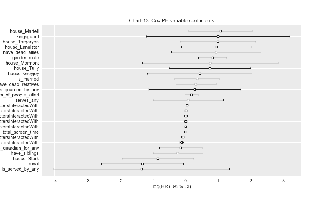
The summary statistics above indicates the significance of each covariate in predicting the survival probabilities. The values under exp(coef) are called hazard ratios (HR). We can interpret HR value as below:
- HR=1: No effect
- HR<1: Reduction in Hazard, meaning more safe.
- HR>1: Increase in Hazard, meaning more risk.
Based on above interpretation, we can make the following observations from the summary above:
- If the character is kingsguard or have dead relatives or of gender male or belongs to any of the houses such as Lannister, Targaryen etc all have high risk because the HR ratios for all of them are above 2.
- total_screen_time seems to have no effect at all as HR=1
- if the character is royal or is served by any, has less risk because HR<1
Final Predictions for Selected Characters
And then, we reach the final section where we make the actual survival predictions using Cox PH model. Here we have done predictions for only few selected characters, but if you wish you may predict any other characters as well.
df2 = character_df[['character_name']]
df2 = df2.merge(df_dummy, how='outer', left_index=True, right_index=True)
tr_rows = df2[df2.character_name.isin(['Tyrion Lannister','Arya Stark','Cersei Lannister','Jaime Lannister','Jon Snow','Sansa Stark','Daenerys Targaryen'])]
tr_rows = tr_rows.set_index('character_name')
cph.predict_survival_function(tr_rows).plot(use_index=False)
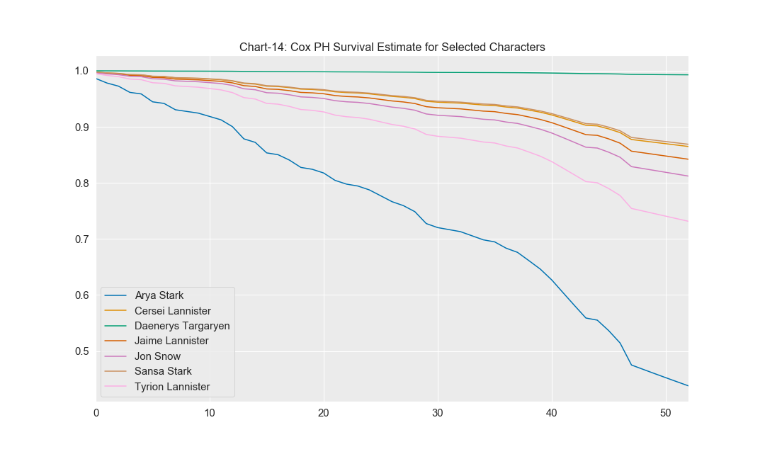
From the chart above:
- Arya Stark and Tyrion Lannister has lesser chance of survival when compared to others. Its quite interesting for Arya because being belonging to Starks should carry lesser risk, but on the other hand she might have buckled up some risk associated in other factors such as number of people killed, have dead relatives etc.
- Daenerys has very highest chances of survival.
- Interestingly Jaime and Cersei have less risk as well.
Below are the survival probabilities and cumulative hazard scores for the selected characters.
cph.predict_cumulative_hazard(tr_rows,[67])
Arya Stark            0.825995
Cersei Lannister      0.145188
Daenerys Targaryen    0.007223
Jaime Lannister       0.171814
Jon Snow              0.208163
Sansa Stark           0.140605
Tyrion Lannister      0.312760
cph.predict_survival_function(tr_rows, [67])
Arya Stark            0.437799
Cersei Lannister      0.864859
Daenerys Targaryen    0.992803
Jaime Lannister       0.842136
Jon Snow              0.812075
Sansa Stark           0.868832
Tyrion Lannister      0.731425
Disclaimer & Code
Please note that the results published in this case study are solely based on my data analysis and the code I wrote. As GoT has full of twists and surprises, these predictions may not hold good in certain scenarios, this blog is just to be used for educational purpose only but not to make any solid conclusion. If you find any error in the analysis, please feel free to bring it to my notice. Also, please feel free to express any concerns or send in any questions or comments.
All the code used in this analysis can be downloaded from this github repository
Leave a comment